Recovering information from a PDF map
2023-02-23This post is going to be about a question that recently came up in the GDAL Matrix room. A user had a discrete heat map of noise levels in their town as a PDF, and wanted to extract some usable information out of it. Let's see if we can help them.
Looking at the data
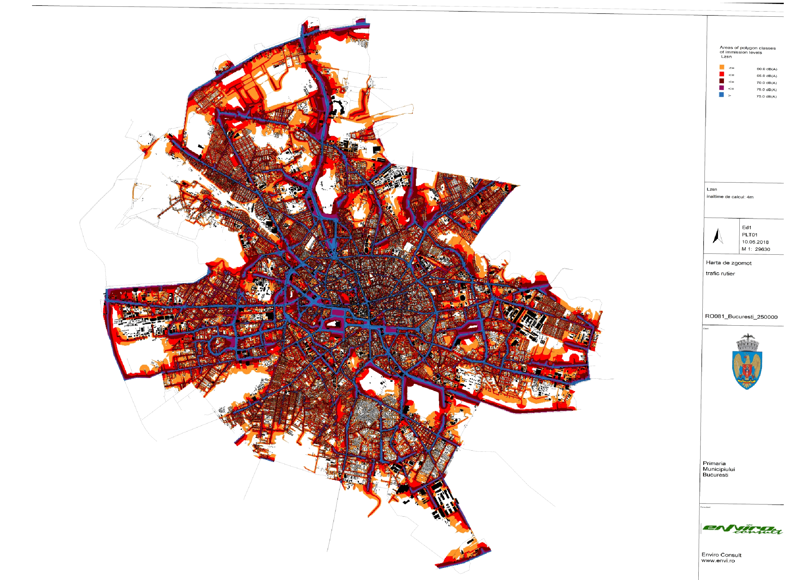
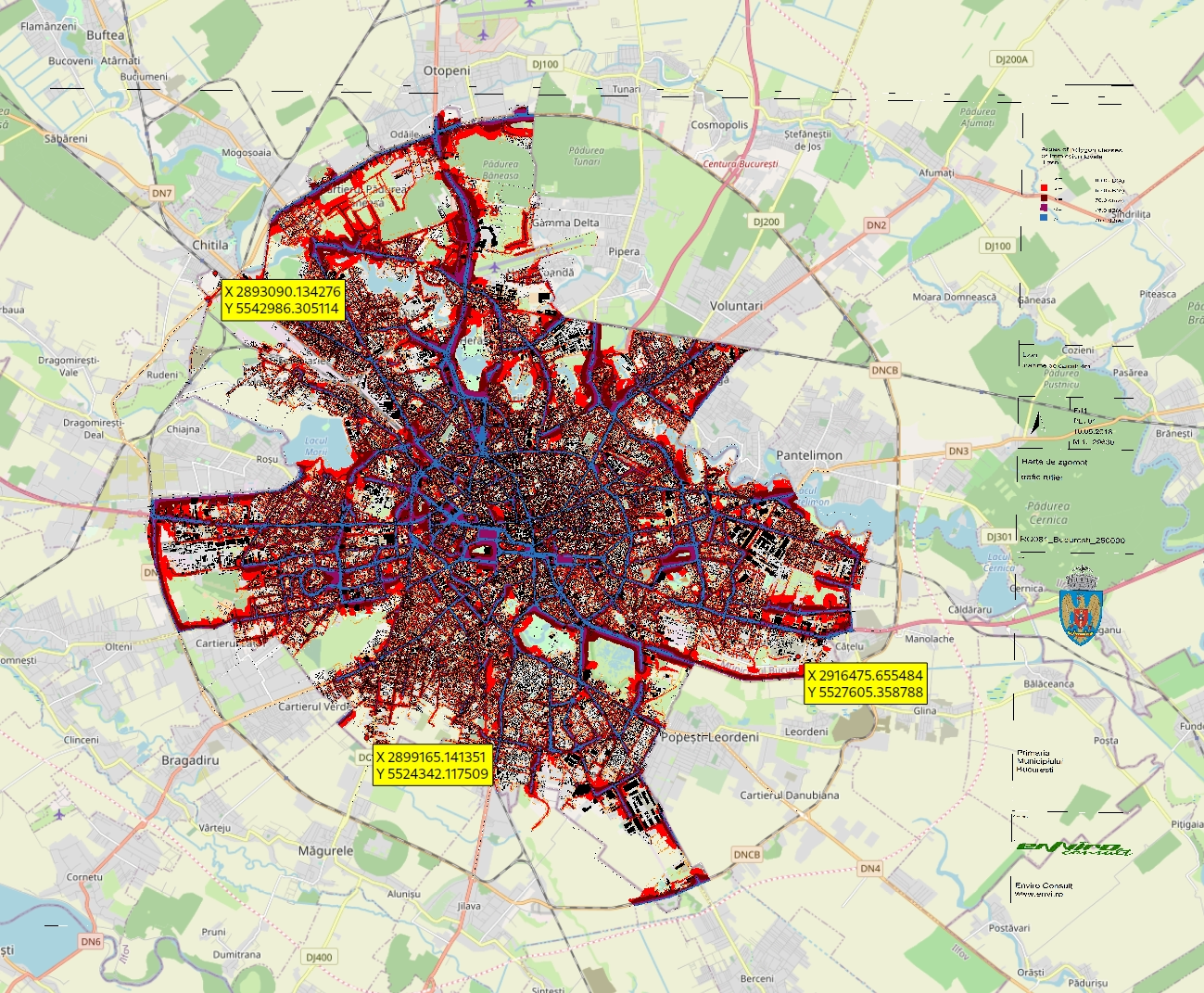
If you want to play along, you can download the file from here. Pick the first one, with Lzsn in its name. It's a 42 MB PDF, looking like this (click on the image for a better version):
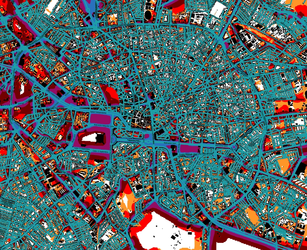
If that seems unreadable, it's partly because my PDF viewer can't zoom into large documents. A better choice is probably QGIS, so you can install it.
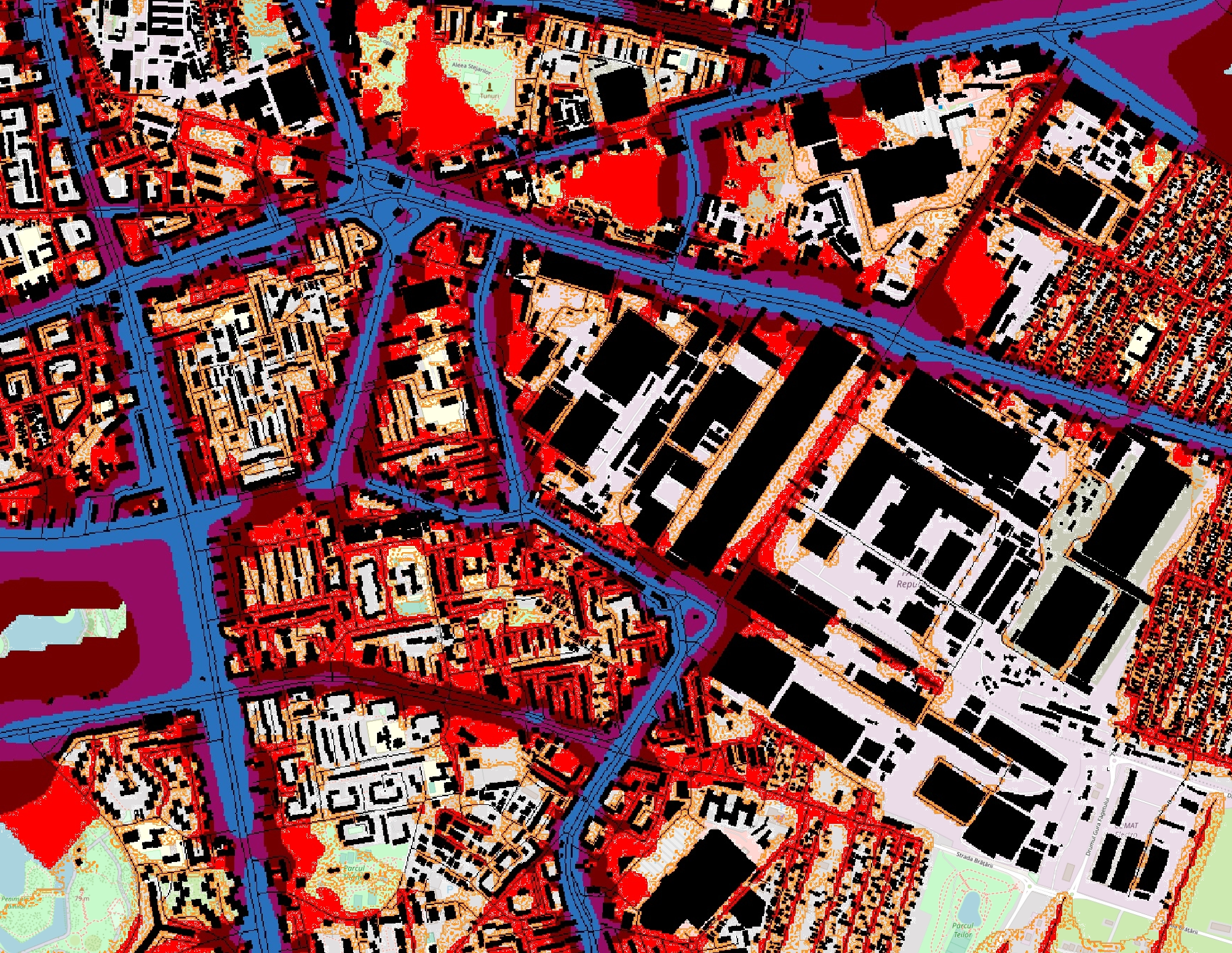
This would probably make a real cartographer unhappy, but fortunately I'm not one. And yes, some labels are doubled, don't ask me why. It happens in Evince, Okular and QGIS, but I don't have a "real" PDF reader to test with.
If you're following along, you might have noticed that QGIS took about 20 minutes to open the file and probably just as long to close it. That's not great and puts our software in a bad light, so let's convert it to a better format.
Using GDAL, you can convert it to a GeoTIFF like this:
$ gdal_translate drumuri_Lzsn.pdf drumuri_Lzsn_temp.tif
$ gdal_translate -f COG -co NUM_THREADS=ALL_CPUS drumuri_Lzsn_temp.tif drumuri_Lzsn.tif
A COG is just a GeoTIFF laid out so it can load faster while zooming in. If you're wondering why I'm doing the conversion in two steps, it just happens to be very slow otherwise, while the commands above should only take a couple of seconds. COGs are tiled (stored in blocks), and going from a striped (stored by lines) to a tiled layout can be slow, but I don't think that's the case for our PDF. Anyway, once you have a TIFF, QGIS should be quite snappy.
Extracting the image
The user would like to have a nice vector dataset, and overlay it on top of OpenStreetMap. This means that we're not really interested in the roads, road labels and building footprints, which are already available there.
I initially missed this, but the user pointed out that the roads in the PDF seem to be stored in a vector format. Maybe there's a chance we can get rid of them?
After some searching, I found the pdfimages tool, part of Poppler.
$ pdfimages -list drumuri_Lzsn.pdf
page   num  type   width height color comp bpc  enc interp  object ID x-ppi y-ppi size ratio
--------------------------------------------------------------------------------------------
   1     0 image   16377 12649  rgb     3   8  jpeg   no         7  0   200   200 39.7M 6.7%
This sounds promising, as we have a large image which we can extract. It's a JPEG, which might cause us some problems later, but we'll cross that bridge when we get there.
$ pdfimages -j drumuri_Lzsn.pdf drumuri_Lzsn
$ ls -lh drumuri_Lzsn*.jpg
-rw-r--r-- 1 user group 40M Feb 21 19:04 drumuri-Lzsn.jpg
$ gdal_translate -f COG -co NUM_THREADS=ALL_CPUS drumuri-Lzsn.jpg drumuri_Lzsn-data.tif
Yes, GDAL can read JPEG, that's pretty nifty. Let's see what we got:
Yup, we still have the legend and other stuff on the right, and we can reasonably suspect that our map was scanned. But is it at least cleaner?
Success — it looks like we're on the right track! We still have the building footprints, but the labels are gone. We won't miss them.
Georeferencing
Unfortunately, if we open both images in QGIS, they won't show up in the same place. This is because the one we extracted is missing the georeferencing and projection information. To put it differently, QGIS doesn't know where the image is located, its orientation and how large a pixel is on the ground.
The original PDF had this information, and it was propagated to the TIFF we made from it:
$ gdalinfo drumuri_Lzsn.tif
Driver: GTiff/GeoTIFF
Files: drumuri_Lzsn.tif
Size is 12992, 9448
Coordinate System is:
PROJCRS["WGS 84 / Pseudo-Mercator",
    BASEGEOGCRS["WGS 84",
        ENSEMBLE["World Geodetic System 1984 ensemble",
            MEMBER["World Geodetic System 1984 (Transit)"],
            MEMBER["World Geodetic System 1984 (G730)"],
            MEMBER["World Geodetic System 1984 (G873)"],
            MEMBER["World Geodetic System 1984 (G1150)"],
            MEMBER["World Geodetic System 1984 (G1674)"],
            MEMBER["World Geodetic System 1984 (G1762)"],
            MEMBER["World Geodetic System 1984 (G2139)"],
            ELLIPSOID["WGS 84",6378137,298.257223563,
                LENGTHUNIT["metre",1]],
            ENSEMBLEACCURACY[2.0]],
        PRIMEM["Greenwich",0,
            ANGLEUNIT["degree",0.0174532925199433]],
        ID["EPSG",4326]],
    CONVERSION["Popular Visualisation Pseudo-Mercator",
        METHOD["Popular Visualisation Pseudo Mercator",
            ID["EPSG",1024]],
        PARAMETER["Latitude of natural origin",0,
            ANGLEUNIT["degree",0.0174532925199433],
            ID["EPSG",8801]],
        PARAMETER["Longitude of natural origin",0,
            ANGLEUNIT["degree",0.0174532925199433],
            ID["EPSG",8802]],
        PARAMETER["False easting",0,
            LENGTHUNIT["metre",1],
            ID["EPSG",8806]],
        PARAMETER["False northing",0,
            LENGTHUNIT["metre",1],
            ID["EPSG",8807]]],
    CS[Cartesian,2],
        AXIS["easting (X)",east,
            ORDER[1],
            LENGTHUNIT["metre",1]],
        AXIS["northing (Y)",north,
            ORDER[2],
            LENGTHUNIT["metre",1]],
    USAGE[
        SCOPE["Web mapping and visualisation."],
        AREA["World between 85.06°S and 85.06°N."],
        BBOX[-85.06,-180,85.06,180]],
    ID["EPSG",3857]]
Data axis to CRS axis mapping: 1,2
Origin = (2886267.104982524644583,5550384.975221752189100)
Pixel Size = (3.554565159517144,-3.554573706431164)
Metadata:
  AREA_OR_POINT=Area
  CREATION_DATE=D:20180606221414
  CREATOR=þÿ
  NEATLINE=POLYGON ((2886267.10498252 5550384.38278758,2886267.10498252 5516801.36284339,2932447.42309224 5516801.36284339,2932447.42309224 5550384.38278758,2886267.10498252 5550384.38278758))
  PRODUCER=Qt 4.8.5 (C) 2011 Nokia Corporation and/or its subsidiary(-ies)
  TITLE=þÿ
Image Structure Metadata:
  COMPRESSION=LZW
  INTERLEAVE=PIXEL
  LAYOUT=COG
Corner Coordinates:
Upper Left  ( 2886267.105, 5550384.975) ( 25d55'40.00"E, 44d32'46.88"N)
Lower Left  ( 2886267.105, 5516801.363) ( 25d55'40.00"E, 44d19'51.43"N)
Upper Right ( 2932448.016, 5550384.975) ( 26d20'33.46"E, 44d32'46.88"N)
Lower Right ( 2932448.016, 5516801.363) ( 26d20'33.46"E, 44d19'51.43"N)
Center      ( 2909357.560, 5533593.169) ( 26d 8' 6.73"E, 44d26'19.51"N)
Band 1 Block=512x512 Type=Byte, ColorInterp=Red
  Min=0.000 Max=255.000
  Minimum=0.000, Maximum=255.000, Mean=222.565, StdDev=77.753
  Overviews: 6496x4724, 3248x2362, 1624x1181, 812x590, 406x295
  Metadata:
    STATISTICS_APPROXIMATE=YES
    STATISTICS_MAXIMUM=255
    STATISTICS_MEAN=222.56487158937
    STATISTICS_MINIMUM=0
    STATISTICS_STDDEV=77.753237328653
    STATISTICS_VALID_PERCENT=100
Band 2 Block=512x512 Type=Byte, ColorInterp=Green
  Min=0.000 Max=255.000
  Minimum=0.000, Maximum=255.000, Mean=214.219, StdDev=83.659
  Overviews: 6496x4724, 3248x2362, 1624x1181, 812x590, 406x295
  Metadata:
    STATISTICS_APPROXIMATE=YES
    STATISTICS_MAXIMUM=255
    STATISTICS_MEAN=214.21891418763
    STATISTICS_MINIMUM=0
    STATISTICS_STDDEV=83.65912385424
    STATISTICS_VALID_PERCENT=100
Band 3 Block=512x512 Type=Byte, ColorInterp=Blue
  Min=0.000 Max=255.000
  Minimum=0.000, Maximum=255.000, Mean=211.690, StdDev=87.032
  Overviews: 6496x4724, 3248x2362, 1624x1181, 812x590, 406x295
  Metadata:
    STATISTICS_APPROXIMATE=YES
    STATISTICS_MAXIMUM=255
    STATISTICS_MEAN=211.69040207532
    STATISTICS_MINIMUM=0
    STATISTICS_STDDEV=87.03195681233
    STATISTICS_VALID_PERCENT=100
You can see it's using EPSG:3857 "Web Mercator" as the coordinate reference system. This tells QGIS and other software how to convert the coordinates in the image to latitude and longitude on the globe. Just below we also have the corner coordinates and pixel spacing (size), which is about 3.55 meters or 3.89 yards.
But the image we extracted using pdfimages doesn't have this information:
$ gdalinfo drumuri_Lzsn-data.tif
Driver: GTiff/GeoTIFF
Files: drumuri_Lzsn-data.tif
Size is 16377, 12649
Image Structure Metadata:
  COMPRESSION=LZW
  INTERLEAVE=PIXEL
  LAYOUT=COG
Corner Coordinates:
Upper Left  (    0.0,    0.0)
Lower Left  (    0.0,12649.0)
Upper Right (16377.0,    0.0)
Lower Right (16377.0,12649.0)
Center      ( 8188.5, 6324.5)
Band 1 Block=512x512 Type=Byte, ColorInterp=Red
  Overviews: 8189x6325, 4095x3163, 2048x1582
Band 2 Block=512x512 Type=Byte, ColorInterp=Green
  Overviews: 8189x6325, 4095x3163, 2048x1582
Band 3 Block=512x512 Type=Byte, ColorInterp=Blue
  Overviews: 8189x6325, 4095x3163, 2048x1582
So what do we do? Can we copy it from the original one? Sure, and it's quite easy!
$ python
Python 3.10.9 (main, Dec 24 2022, 19:48:26) [GCC 12.2.0] on linux
Type "help", "copyright", "credits" or "license" for more information.
>>> from osgeo import gdal
>>> image = gdal.Open("drumuri_Lzsn-data.tif")
>>> reference = gdal.Open("drumuri_Lzsn.tif")
>>> reference.GetProjection() # just to check
'PROJCS["WGS 84 / Pseudo-Mercator",GEOGCS["WGS 84",DATUM["WGS_1984",SPHEROID["WGS 84",6378137,298.257223563,AUTHORITY["EPSG","7030"]],AUTHORITY["EPSG","6326"]],PRIMEM["Greenwich",0,AUTHORITY["EPSG","8901"]],UNIT["degree",0.0174532925199433,AUTHORITY["EPSG","9122"]],AUTHORITY["EPSG","4326"]],PROJECTION["Mercator_1SP"],PARAMETER["central_meridian",0],PARAMETER["scale_factor",1],PARAMETER["false_easting",0],PARAMETER["false_northing",0],UNIT["metre",1,AUTHORITY["EPSG","9001"]],AXIS["Easting",EAST],AXIS["Northing",NORTH],EXTENSION["PROJ4","+proj=merc +a=6378137 +b=6378137 +lat_ts=0 +lon_0=0 +x_0=0 +y_0=0 +k=1 +units=m +nadgrids=@null +wktext +no_defs"],AUTHORITY["EPSG","3857"]]'
>>> reference.GetGeoTransform() # just to check
(2886267.1049825246, 3.5545651595171437, 0.0, 5550384.975221752, 0.0, -3.5545737064311638)
>>> image.SetProjection(reference.GetProjection())
0
>>> image.SetGeoTransform(reference.GetGeoTransform())
0
>>> image.FlushCache() # write our changes to disk

$ gdalinfo drumuri_Lzsn-data.tif
Driver: GTiff/GeoTIFF
Files: drumuri_Lzsn-data.tif
       drumuri_Lzsn-data.tif.aux.xml
Size is 16377, 12649
Coordinate System is:
PROJCRS["WGS 84 / Pseudo-Mercator",
    BASEGEOGCRS["WGS 84",
        DATUM["World Geodetic System 1984",
            ELLIPSOID["WGS 84",6378137,298.257223563,
                LENGTHUNIT["metre",1]]],
        PRIMEM["Greenwich",0,
            ANGLEUNIT["degree",0.0174532925199433]],
        ID["EPSG",4326]],
    CONVERSION["unnamed",
        METHOD["Popular Visualisation Pseudo Mercator",
            ID["EPSG",1024]],
        PARAMETER["Latitude of natural origin",0,
            ANGLEUNIT["degree",0.0174532925199433],
            ID["EPSG",8801]],
        PARAMETER["Longitude of natural origin",0,
            ANGLEUNIT["degree",0.0174532925199433],
            ID["EPSG",8802]],
        PARAMETER["False easting",0,
            LENGTHUNIT["metre",1],
            ID["EPSG",8806]],
        PARAMETER["False northing",0,
            LENGTHUNIT["metre",1],
            ID["EPSG",8807]]],
    CS[Cartesian,2],
        AXIS["easting",east,
            ORDER[1],
            LENGTHUNIT["metre",1]],
        AXIS["northing",north,
            ORDER[2],
            LENGTHUNIT["metre",1]],
    ID["EPSG",3857]]
Data axis to CRS axis mapping: 1,2
Origin = (2886267.104982524644583,5550384.975221752189100)
Pixel Size = (3.554565159517144,-3.554573706431164)
Image Structure Metadata:
  COMPRESSION=LZW
  INTERLEAVE=PIXEL
  LAYOUT=COG
Corner Coordinates:
Upper Left  ( 2886267.105, 5550384.975) ( 25d55'40.00"E, 44d32'46.88"N)
Lower Left  ( 2886267.105, 5505423.172) ( 25d55'40.00"E, 44d15'28.05"N)
Upper Right ( 2944480.219, 5550384.975) ( 26d27' 2.58"E, 44d32'46.88"N)
Lower Right ( 2944480.219, 5505423.172) ( 26d27' 2.58"E, 44d15'28.05"N)
Center      ( 2915373.662, 5527904.074) ( 26d11'21.29"E, 44d24' 8.11"N)
Band 1 Block=512x512 Type=Byte, ColorInterp=Red
  Overviews: 8189x6325, 4095x3163, 2048x1582
Band 2 Block=512x512 Type=Byte, ColorInterp=Green
  Overviews: 8189x6325, 4095x3163, 2048x1582
Band 3 Block=512x512 Type=Byte, ColorInterp=Blue
  Overviews: 8189x6325, 4095x3163, 2048x1582
If you're wondering, the "Geotransform" is a set of parameters for an affine transformation. It can describe a combination of translation (where the image is located), scaling (how large a pixel is), rotation (the orientation of the image) and shear, which I suspect nobody uses. These are sufficient for any "well-behaved" image like those you'll find on my blog, but that's not always the case.
We can load them both in QGIS, but something seems a little off. In the screenshot below, I reduced the transparency of drumuri_Lzsn-data.tif:

That's pretty awful, and it seems that our approach was not quite right. In retrospect, this makes sense. The PDF had a correct georeference, but it doesn't necessarily transfer to the one we extracted, because we didn't take into account the position and scale of the image on the page.
Georeferencing, again
Fortunately, not all is lost, as this must be a problem a lot of QGIS users must running into. Digitizing a map doesn't seem like such a rare use case, and I knew that QGIS has a feature that helps with this. What we'd like to do is pick some points on our image, find their pair in the original one, and let QGIS figure it out. In GIS-speak, these are called GCPs, for Ground Control Points.
We can do this using the Georeferencer tool. If you're looking it up, a lot of documentation online is outdated, and it's now found Layer menu. The documentation makes this seem pretty complex, but it's not that bad.
Note: if you're following along, the file you load must not have a geotransform, otherwise QGIS will get very confused. So we have to undo the work from the previous section. The easiest way is probably to rebuild the file:
$ gdal_translate -f COG -co NUM_THREADS=ALL_CPUS drumuri-Lzsn.jpg drumuri_Lzsn-data.tif
I opened the tool, loaded the raster (drumuri_Lzsn-data.tif), then zoomed in a lot and clicked on a pixel that seemed easy to spot. A new window showed up asking for some coordinates, I clicked "From Map Canvas" and selected the corresponding pixel from the original (drumuri_Lzsn-data.tif):
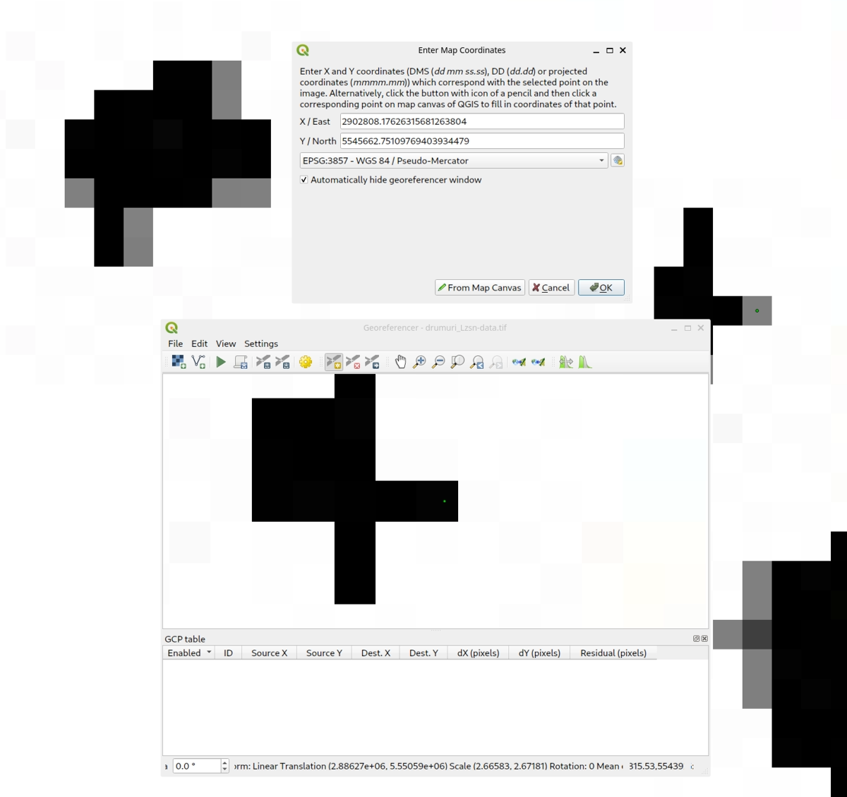
The points you click on don't get snapped to pixel centers, so I tried to be somewhat precise when clicking.
After hitting "OK", the GCP showed up at the bottom of the window.
You need at least two pairs of points, but I picked three because it was pretty fun. It's probably a good idea to choose points that are far apart from each other.
Then I went to "Transformation Settings", checked "Set target resolution", but left the horizontal and vertical values set to 0 (you get a weird error if you don't do this). Linear and Nearest Neighbor should be fine. Once you hit start, you should see a drumuri_Lzsn-data_modified.tif layer in QGIS.
Here I opened the layer settings and added 255 as an additional no data value in the Transparency tab, then added the OpenStreetMap XYZ tileset:
Unfortunately, I couldn't get a pixel-perfect match over the original, but it should be good enough for practical purposes.
Next steps
Our result looks encouraging, but we still need to do something about the compression artefacts (remember, the image we extracted is a JPEG) and, ideally, fill in the building footprints. If you'd like to read more, stay tuned for the next part!